Tidy tuesday 20-01-14 : the passwords dataset
tt_20-01-14_passwords.RmdData import and inspection
One can obtain the metadata table using datapasta’s R package addin and copying the table available at
meta <- data.frame(stringsAsFactors=FALSE,
                   variable = c("rank", "password", "category", "value", "time_unit",
                                "offline_crack_sec", "rank_alt", "strength", "font_size"),
                   class = c("double", "character", "character", "double", "character",
                             "double", "double", "double", "double"),
                   description = c("popularity in their database of released passwords",
                                   "Actual text of the password",
                                   "What category does the password fall in to?", "Time to crack by online guessing",
                                   "Time unit to match with value", "Time to crack offline in seconds",
                                   "Rank 2", "Strength = quality of password where 10 is highest,
                   1 is lowest,
                   please note that these are relative to these generally bad passwords", "Used to create the graphic for KIB")
)
meta <- as_tibble(meta)

pander::pander(meta)| variable | class | description |
|---|---|---|
| rank | double | popularity in their database of released passwords |
| password | character | Actual text of the password |
| category | character | What category does the password fall in to? |
| value | double | Time to crack by online guessing |
| time_unit | character | Time unit to match with value |
| offline_crack_sec | double | Time to crack offline in seconds |
| rank_alt | double | Rank 2 |
| strength | double | Strength = quality of password where 10 is highest, 1 is lowest, please note that these are relative to these generally bad passwords |
| font_size | double | Used to create the graphic for KIB |
the readr::read_csv function gives some information on how the data was processed, with here no errors or warnings.
passwords <- readr::read_csv('https://raw.githubusercontent.com/rfordatascience/tidytuesday/master/data/2020/2020-01-14/passwords.csv')
#> Parsed with column specification:
#> cols(
#>   rank = col_double(),
#>   password = col_character(),
#>   category = col_character(),
#>   value = col_double(),
#>   time_unit = col_character(),
#>   offline_crack_sec = col_double(),
#>   rank_alt = col_double(),
#>   strength = col_double(),
#>   font_size = col_double()
#> )
The passwords dataset has 507 rows * 9 variables. It is not tidy, if we want to use the value variable of online guessing we need to add the time_unit information to it.
passwords %>%
  glimpse()
#> Observations: 507
#> Variables: 9
#> $ rank              <dbl> 1, 2, 3, 4, 5, 6, 7, 8, 9, 10, 11, 12, 13, 1...
#> $ password          <chr> "password", "123456", "12345678", "1234", "q...
#> $ category          <chr> "password-related", "simple-alphanumeric", "...
#> $ value             <dbl> 6.91, 18.52, 1.29, 11.11, 3.72, 1.85, 3.72, ...
#> $ time_unit         <chr> "years", "minutes", "days", "seconds", "days...
#> $ offline_crack_sec <dbl> 2.17e+00, 1.11e-05, 1.11e-03, 1.11e-07, 3.21...
#> $ rank_alt          <dbl> 1, 2, 3, 4, 5, 6, 7, 8, 9, 10, 11, 12, 13, 1...
#> $ strength          <dbl> 8, 4, 4, 4, 8, 4, 8, 4, 7, 8, 8, 1, 32, 9, 9...
#> $ font_size         <dbl> 11, 8, 8, 8, 11, 8, 11, 8, 11, 11, 11, 4, 23...
Glimpse of the passwords :
| rank | password | category | value | time_unit | offline_crack_sec |
|---|---|---|---|---|---|
| 1 | password | password-related | 6.91 | years | 2.17 |
| 2 | 123456 | simple-alphanumeric | 18.52 | minutes | 1.11e-05 |
| 3 | 12345678 | simple-alphanumeric | 1.29 | days | 0.00111 |
| 4 | 1234 | simple-alphanumeric | 11.11 | seconds | 1.11e-07 |
| 5 | qwerty | simple-alphanumeric | 3.72 | days | 0.00321 |
| 6 | 12345 | simple-alphanumeric | 1.85 | minutes | 1.11e-06 |
| rank_alt | strength | font_size |
|---|---|---|
| 1 | 8 | 11 |
| 2 | 4 | 8 |
| 3 | 4 | 8 |
| 4 | 4 | 8 |
| 5 | 8 | 11 |
| 6 | 4 | 8 |
Quality check
# --- using base R function
# passwords %>%
#   qual_fun(.)

# --- tidyverse approach
passwords %>%
  tidy_qual() %>%
pander::pander()| indic | rank | password | category | value | time_unit | offline_crack_sec |
|---|---|---|---|---|---|---|
| n_na | 7 | 7 | 7 | 7 | 7 | 7 |
| n_nan | 0 | 0 | 0 | 0 | 0 | 0 |
| n_inf | 0 | 0 | 0 | 0 | 0 | 0 |
| rank_alt | strength | font_size |
|---|---|---|
| 7 | 7 | 7 |
| 0 | 0 | 0 |
| 0 | 0 | 0 |
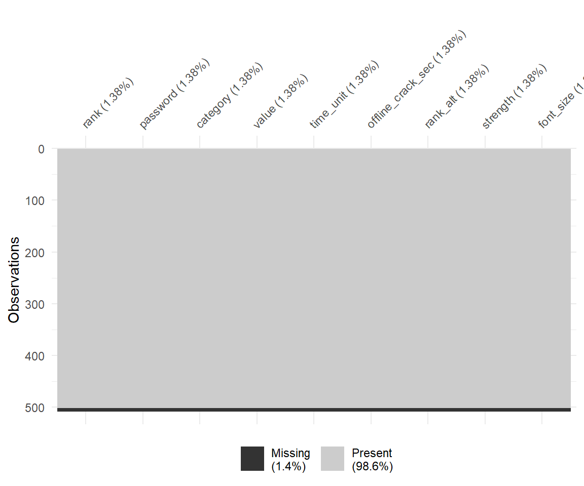
The 7 missing values are the in the same rows :
passwords %>%
  filter(!complete.cases(passwords))
#> # A tibble: 7 x 9
#>    rank password category value time_unit offline_crack_s~ rank_alt
#>   <dbl> <chr>    <chr>    <dbl> <chr>                <dbl>    <dbl>
#> 1    NA <NA>     <NA>        NA <NA>                    NA       NA
#> 2    NA <NA>     <NA>        NA <NA>                    NA       NA
#> 3    NA <NA>     <NA>        NA <NA>                    NA       NA
#> 4    NA <NA>     <NA>        NA <NA>                    NA       NA
#> 5    NA <NA>     <NA>        NA <NA>                    NA       NA
#> 6    NA <NA>     <NA>        NA <NA>                    NA       NA
#> 7    NA <NA>     <NA>        NA <NA>                    NA       NA
#> # ... with 2 more variables: strength <dbl>, font_size <dbl>
In total those missing values represent less than 2% of the total of data.
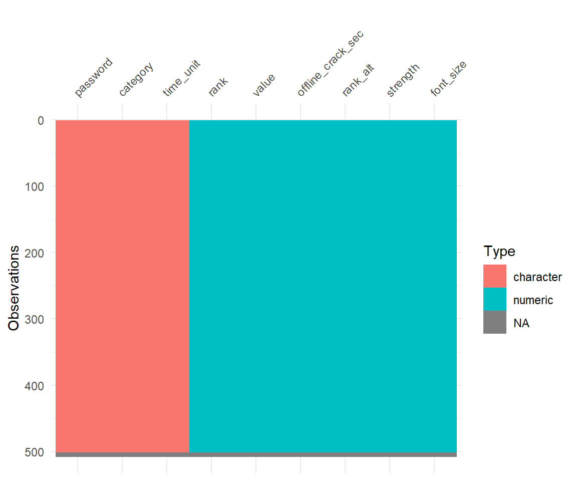
Cleaning
To fix the types, the character variables are set as factors.
psw_clean <-
  passwords %>%
  filter(complete.cases(passwords)) %>%
  mutate_if(is.character, factor) %>%
  tidyr::unite(data = ., col = "online_duration", value, time_unit, sep = " ", remove = FALSE) %>%
  mutate(online_duration = lubridate::duration(num = online_duration),
         od_num = as.numeric(online_duration)
  )
The value and time unit are united in the online_time variable with seconds as unit.
# summary(psw_clean)
log_df <- tibble(
  unit = c("sec", "min", "h", "day", "week", "month", "year", "10years", "100years"),
  logv = log(c( 1, 60, 3600, 24*3600, 7*24*3600, 30*24*3600,
                365.25*24*3600, 10*365.25*24*3600, 100*365.25*24*3600) ),
  y = 0.65
)

# exp(30)/(20*365.25*24*3600)

psw_clean %>%
  ggplot(aes(x = log(od_num), y = stat(density))) +
  geom_histogram() +
  geom_vline(xintercept = log_df$logv, colour = "red") +
  geom_label(data = log_df, aes(x = logv, y = y, label = unit)) + # inherit.aes = FALSE,
  theme_light() + xlab("log(duration)") + ylab("Density") +
  ggtitle("Density historam of the log duration to hack passwords")
#> `stat_bin()` using `bins = 30`. Pick better value with `binwidth`.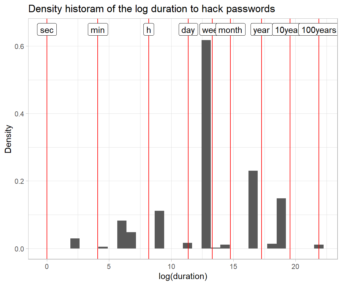
Univariate study
There are 10 unique categories and 7 unit of time. Passwords are unique individuals in this dataset.
psw_clean %>%
  summarise_if(.tbl = .,.predicate = is.factor, .funs = list("nb_u" = ~length(unique(.))) ) %>%
  mutate(indic = "nb unique") %>%
  select(indic, everything())
#> # A tibble: 1 x 4
#>   indic     password_nb_u category_nb_u time_unit_nb_u
#>   <chr>             <int>         <int>          <int>
#> 1 nb unique           500            10              7
1/3 of the passwords are names, most are actually dictionnary words.
cat_stat <- psw_clean %>%
  group_by(category) %>%
  summarise(nb = n(),
            pct = nb/nrow(psw_clean)*100) %>%
  arrange(-nb)

cat_stat %>%
  ggplot(aes(x = forcats::fct_reorder(.f = category, .x = pct), y = pct)) +
  geom_col(fill = "#4F62DB") +
  geom_text(aes(y = pct + 2, label = pct), size = 4) +
  xlab("Category of passord") + ylab("Percentage") +
  ggtitle("Repartition of the passwords per categories") +
  theme_light() +
  coord_flip()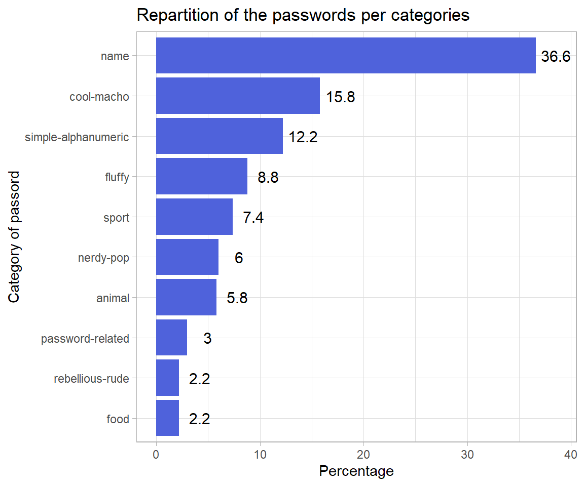
Nearly 70% of the passwords considered are crackable online in less than a week, 20% are guessable within a day.
tu_stat <- psw_clean %>%
  group_by(time_unit) %>%
  summarise(nb = n(),
            pct = nb/nrow(psw_clean)*100) %>%
  arrange(-nb)

tu_stat %>%
  ggplot(aes(x = forcats::fct_reorder(.f = time_unit, .x = pct), y = pct)) +
  geom_col(fill = "#D91515") +
  geom_text(aes(y = pct + 2, label = pct)) +
  xlab("Time unit to crack a passord") + ylab("Percentage") +
  ggtitle("Repartition of the time unit required to crack passwords") +
  theme_light() +
  coord_flip()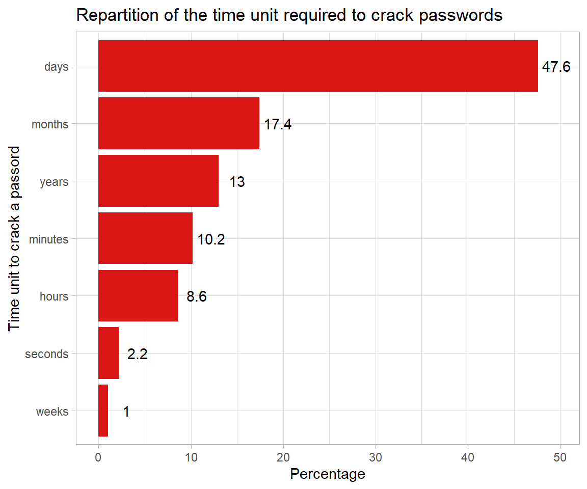
We can look at the character type distribution in the passwords.
library(stringr)

passwd_type <- psw_clean %>%
  mutate(password = as.character(password)) %>%
  mutate("nb_char" = nchar(password),
         num_part = purrr::map_chr( stringr::str_extract_all(string = password, pattern = "[:digit:]"),
                                    function(x) paste(x, collapse = "") ),
         nchar_num = nchar(num_part),

         alpha_part = purrr::map_chr( stringr::str_extract_all(string = password, pattern = "[:alpha:]"),
                                      function(x) paste(x, collapse = "") ),
         nchar_alpha = nchar(alpha_part),

         punct_part = purrr::map_chr( stringr::str_extract_all(string = password, pattern = "[:punct:]"),
                                      function(x) paste(x, collapse = "") ),
         nchar_punct = nchar(punct_part),

         lower_part = purrr::map_chr( stringr::str_extract_all(string = password, pattern = "[:lower:]"),
                                      function(x) paste(x, collapse = "") ),
         nchar_lower = nchar(lower_part),

         upper_part = purrr::map_chr( stringr::str_extract_all(string = password, pattern = "[:upper:]"),
                                      function(x) paste(x, collapse = "") ),
         nchar_upper = nchar(upper_part)
  )
The data contains passwords with numeric and alpha character. All of alpha character use lower case.
| variable | mean | var | sd | min | 1q | median | 3q | max |
|---|---|---|---|---|---|---|---|---|
| nchar_num | 0.54 | 2.79 | 1.67 | 0 | 0 | 0 | 0 | 9 |
| nchar_alpha | 5.66 | 3.88 | 1.97 | 0 | 6 | 6 | 7 | 8 |
| nchar_punct | 0 | 0 | 0 | 0 | 0 | 0 | 0 | 0 |
| nchar_lower | 5.66 | 3.88 | 1.97 | 0 | 6 | 6 | 7 | 8 |
| nchar_upper | 0 | 0 | 0 | 0 | 0 | 0 | 0 | 0 |
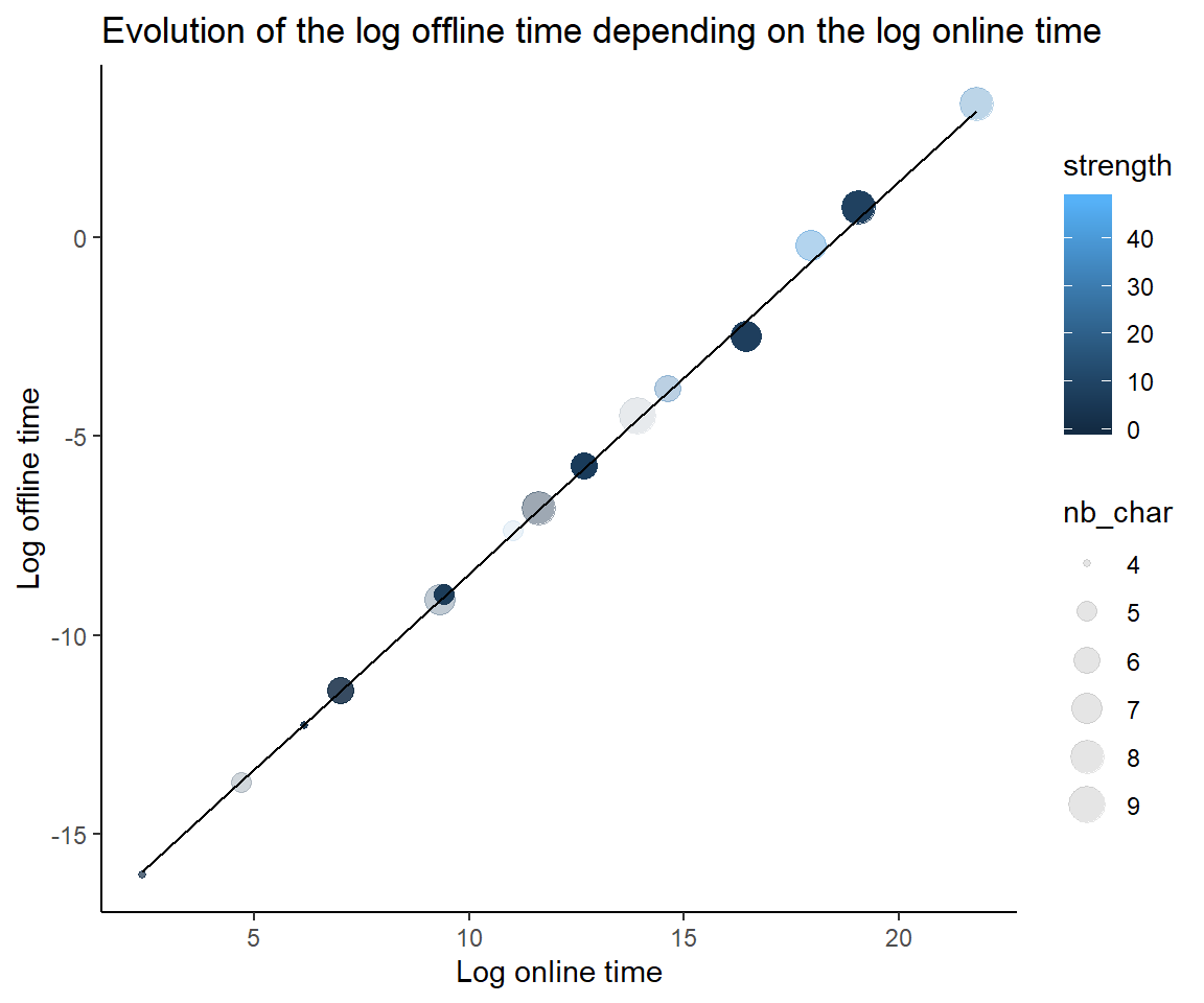
One can suspect a linear relation between the online and offline time of cracking.
# passwd_type %>% View()
passwd_type %>% # glimpse()
  ggplot(aes(x = od_num, y = offline_crack_sec, colour = strength, size = factor(nb_char)) ) +
  geom_point(alpha = .1)
#> Warning: Using size for a discrete variable is not advised.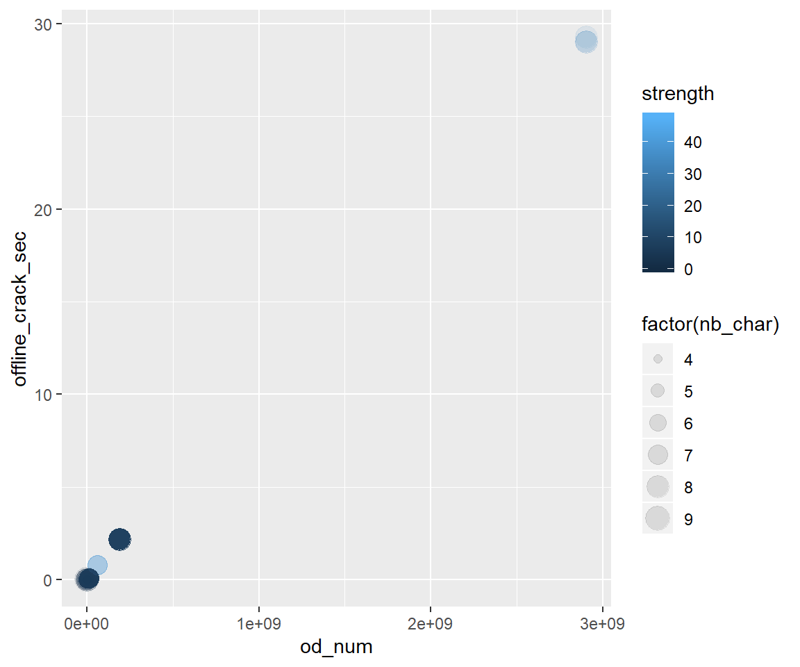
This is confirmed passing to (log ,log) scaled plot. The formula obatined is
\[log(offline) = -18.322 + 0.987 \times log(online)\]
df_min <- passwd_type %>% transmute(x = log(od_num), y = log(offline_crack_sec))
# summary(df_min)
lm_mod <- lm(y ~ x, df_min)
# summary(lm_mod)
df_min$y_hat <- predict.lm(lm_mod, newdata = df_min)

passwd_type %>% # glimpse()
  ggplot(aes(x = log(od_num), y = log(offline_crack_sec), colour = strength, size = nb_char ) ) +
  geom_point(alpha = .1) +
  geom_line(data = df_min, aes(x, y_hat), inherit.aes = FALSE) +
  xlab("Log online time") + ylab("Log offline time") +
  ggtitle("Evolution of the log offline time depending on the log online time") +
  theme_classic()